Brownian motion is the random movement of particles suspended in a fluid, caused by constant collisions with surrounding molecules. This phenomenon, observed at microscopic scales, reflects the principles of diffusion and randomness. Analyzing the movement of particles through techniques like MSD (Mean Square Displacement) reveals insights into diffusion processes.
Objective of the experiment: Estimating Avogadro’s number using Brownian Motion and Verification of number distribution
Observation:
In this experiment, we have observed Brownian motion with polystyrene colloids (size ~ micron) dispersed into water solution. Two drops of the solution were placed on a glass microslide, and the droplets were made airtight using square-cut paraffin paper, lubricant (vaseline), and a transparent coverslip before observing this with a Celestron Pentaview microscope. With the help of the microscope, a one-minute video was recorded for further analysis.
Here is a recorded video of Brownian motion at ICTS (feel free to download this and perform the analysis!)
Theory:
We have used the following theory to determine the Avogadro's number from the observed Brownian motion:
Video Analysis:
From the video, we need to plot the mean square deviation (MSD) of particles as a function of time, and we will be able to get the value of the diffusion constant (D) from the slope of the plot. To do that, we have to know the basics of image processing and familiarity with Python's dedicated openCV library. For those who don't like to work with Python or any other programming language, ImageJ (an image processing software) would be a good start.
How to execute the analysis and get the plot from the recorded video? Watch here
The process of the analysis is briefly described below:
1. At first, we are going to break the video into frames using Python (on Google Collab) or ImageJ.
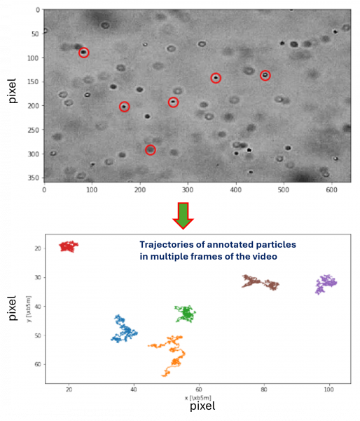
2. Annotating the particles: In a particular frame of the video, we need to find and mark the particles to capture their motion in the video. This process is called annotation. To understand more, see the image below:

3. If we have a 30-second video, it's very likely that not all particles annotated in a specific frame (as shown above) will remain within the rectangular view for the entire duration. Some particles may exit the viewing area after a few seconds and then return later. To ensure accurate analysis, we need to identify and discard particles that leave the view before the 30-second mark. As illustrated below, we've removed the particles that exited early, and will now focus only on those that stayed within the viewing area for the full duration of the video.
4. Next, we have to extract the trajectory of the particles under investigation (see the image below).

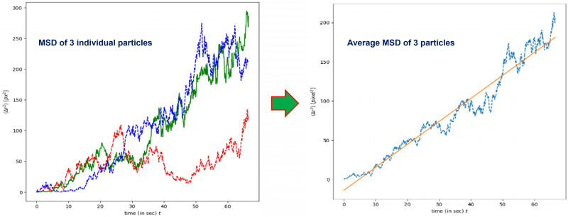
5. Once we have the trajectory of the particles under investigation, we can plot the MSD vs time plot to get the slope and subsequently the value of D (see theory section). To do that, at first, we are going to plot the MSD vs time for individual particles and average it to calculate the slope of the plot. See the figure below to learn more:

From the slope, the calculated value of Avogadro's number is as follows:
Resources:
- Jean Perrin's write-up, Perrin's book
- Trackpy for tracking particles
- More on N
- Details of the experiment
- Polystyrene particles used
Acknowledgments: This experiment has been successful with the help of integrated PhD students at ICTS, Prof. Mahesh Bandi (OIST), & Prof. Abhishek Dhar (ICTS)
PS: If you are trying this experiment or performing the analysis after downloading the video given above and have any questions, don't hesitate to write to me at: ikbal.ahmed@icts.res.in


